Activation Steering vs. Finetuning: How Different Are They Really?

TL;DR

This post investigates the following questions: Where should we steer a model? And how expressive can steering actually be?

By comparing steering and finetuning through a first-order lens, we find that often the best place to steer is after the skip connection, where attention and MLP outputs meet. Steering here is more expressive than steering individual submodules, and it ends up looking a lot closer to what finetuning does. Using this insight, we build lightweight post-block adapters that train only a fraction of the model’s parameters and achieve remarkably close performance to SFT.

Note: This post is aimed at readers comfortable with transformers and some linear algebra. We’ll keep the math light but precise.

The Paradigm: Activation Steering vs. finetuning

Activation steering is an alternative to parameter-efficient finetuning (PEFT). Instead of updating weights, it directly edits a model’s hidden activations at inference time, cutting the number of trainable parameters by an order of magnitude. ReFT [1], for example, reaches LoRA-level performance while using 15×–65× fewer parameters. If we can reliably match finetuning with so few parameters, that changes what’s feasible: we can adapt larger models, run more expensive training objectives, or simply get more done under the same compute budget.

Existing steering methods mainly differ in where they apply these interventions: ReFT modifies MLP outputs (post-MLP), LoFIT [2] steers at attention heads (pre-MLP), and JoLA [3] jointly learns both the steering vectors and the intervention locations.

The Problem: We Are Steering in the Dark

Despite empirical success, we still lack a clear understanding of why steering works and how to reason about where is the best steering location. Two key questions remain open:

1. The Location Dilemma. Why do some steering locations outperform others? And does understanding how activation steering approximates weight updates help reveal which modules are best to steer? (Spoiler: it does)
2. The Expressivity Gap. SFT and LoRA leverage the model’s nonlinear transformations, while most steering methods rely on linear adapters. How much does this limit their ability to mimic the effects of weight updates?

This work investigates both questions.

First: Where should we steer? We begin with a simple, linearized analysis of a GLU’s output changes under weight updates compared to activation steering. This shows us that steering at some locations can easily match the behavior of certain weight updates, but not others. However, we notice that linear steering at these locations cannot completely capture the full behavior of weight updates.

Then: How expressive can steering really be? We then experiment with oracle steering, which, while not a practical method, provides a principled way to test which locations are best to steer at. With this tool, one pattern stands out: the most expressive intervention point is the block output, after the skip connection. Steering here can draw on both the skip-connection input and the transformed MLP output, instead of relying solely on either the MLP or attention pathway.

Motivated by this, we introduce a new activation adapter placed at each block output. It retains a LoRA-like low-rank structure but incorporates a non-linearity after the down-projection. This allows it to capture some of the nonlinear effects of SFT, giving activation steering a more expressive update space.

And finally: A bit of theory. No matter what the steering adapter is, if the adapter is able enough to match the fine-tuned model at each layer, the steered model will be able to match the fine-tuned model. So, how accurate must we be to match a fine-tuned model closely?

We also show that, at least in some settings relating to the geometry of these hidden states and the residuals at each module, post-block steering can replicate post-MLP steering. Also, we show that under some (very specific) parameter settings, post-MLP steering cannot learn anything, while post-block steering still can. This can be evolved into an approximation showing that, in broader, more applicable settings, post-MLP steering can get quite close to pre-MLP steering.

Some notation/background

Throughout this article, we will be looking at a number of different places to steer, along with different ways that we can steer. Even if some of these choices don’t make sense at the moment, don’t worry! A lot of this will be explained much more throughout this article. Use this section as a reference for any unclear notation/names as you read.

We will use $\delta\cdot$ to represent small induced changes in our analysis, and $\Delta\cdot$ will represent changes to parameters, such as the finetuning updates to matrices $\Delta W$ or steering vector $\Delta h$.

First, a Transformer model is built from transformer blocks. Each block contains an Attention module and an MLP module. Unless otherwise specified, the MLP modules will be specifically GLU layers, a popular variant of standard 1-layer MLPs. The inputs to each submodule of each layer will pass through a LayerNorm. Each layer will involve two skip-connections, one around each submodule. This all can be seen in the picture below.

As for steering, there are 3 main variants we consider. (1) pre-MLP steering involves steering attention outputs; most commonly done by steering the output of individual attention heads, before skip-connection and normalization; (2) post-MLP steering involves steering the output of the MLP/GLU layer before it goes through the skip-connection; (3) post-block steering involves steering the output of each block, which can be seen as equivalently steering the output of the MLP/GLU layer after it goes through the skip connection. In our notation, a GLU is represented as

The matrices $W_d, W_g, W_u$ are called the down-projection, gated, and up-projection matrices respectively. When convenient, we will also write

For mathematical notation, the hidden state will be represented as a vector $h$ and steering will be represented as $\Delta h$. So, steering works by replacing $h$ with $h + \Delta h$.

Note: $\Delta h$, the steering vector, can depend on the input. Sometimes this is written explicitly as $\Delta h(h)$, but other times it is omitted.

• Fixed-vector: The simplest form of steering is by adding a fixed vector $v$ to the hidden state:

• Linear/ReFT: Linear steering involves some matrix $A$ and bias vector $b$, where the steering vector is a linear function of the hidden state. However, the matrix $A$ is usually replaced by a low-rank matrix (usually written as $W_uW_d^\top$ or $AB^\top$). The rank of this matrix is written as $r$ when necessary:

• Non-linear: This steering is parameterized by a 1-layer MLP with matrices $W_u, W_d$ as the down- and up-projections with SiLU activation $\phi$:

• Freely parametrized/Oracle: In this case, the steering vector has no explicit parameterization. It can depend on the hidden state $h$ in any way. The oracle specifically will be given by the difference between the hidden states of the base and fine-tuned model

With notation in place, we are now ready to begin our analysis!

Where should we steer?

Let’s start with the main question that drives the rest of our analysis:

At which points in the network can steering match the effect of updating the weights in that same module?

We will examine pre-MLP (steering attention outputs, like LoFIT) and post-MLP (steering the MLP output before the skip connection, like ReFT) steering as they are the most common choice in the literature. These spots nicely sandwich the MLP, so the most immediate module affected by steering at these points is the MLP itself. Our first step is simple: compare the output changes caused by steering at these locations to the output changes caused by tuning the MLP weights.

Note: Before we start, it will feel like there is a lot of math here, but we promise, everything in this section is linear algebra.

finetuning

Let the MLP output be

finetuning the weights gives us

The updates $\Delta W_g$ and $\Delta W_u$ induce the following changes in their immediate outputs:

A first order Taylor expansion of $m = \sigma(a_g) \odot a_u$ gives

Plugging in $\delta m$ into finetuning output gives us

This yields the first-order shift caused by finetuning:

Plugging $\delta m$ into $y = W_d m$ gives us

Let’s compare the finetuning and pre-MLP steering output shifts side by side

Notice that the 2nd term in $\delta y_{\mathrm{FT}}$ is structurally similar to $\delta y_{\mathrm{pre}}$. What does this imply?

In principle, pre-MLP steering can match the shift caused by the updates $\Delta W_u$ and $\Delta W_g$, if there exist a $\Delta h$ such that $W_g \Delta h \approx (\Delta W_g) h$ and $W_u \Delta h \approx (\Delta W_u) h$.

Wait, what about the first term $(\Delta W_d) m$? For a $\Delta h$ to match this term, $(\Delta W_d) m$ must lie in a space reachable by pre-MLP steering. Let’s factor out $\Delta h$ to see what that space looks like:

Define $J(h) = (\sigma’(a_g) \odot a_u) \odot W_g + \sigma(a_g) \odot W_u \quad$ and $\quad A(h) = W_d J(h),$ where elementwise-product between a vector and a norm is performed row-wise, i.e. $a \odot W = \mathbf{1}a^\top \odot W$.

We can rewrite \(\delta y_{\mathrm{pre}} = A(h) \Delta h.\)

For pre-MLP steering to match finetuning MLP shift, we must have: \((\Delta W_d) m \in \text{col}(A(h)).\) What does this mean?

• Since $A(h) = W_d J(h) \subseteq \text{col}(W_d)$, any part of $(\Delta W_d) m$ orthogonal to $\text{col}(W_d)$ is unreachable.
• If finetuning pushes $\Delta W_d$ to new directions not spanned by $A(h)$, pre-MLP steering cannot match it.
• Note that as this condition must hold for every token $h$, this becomes really restrictive.

Bottom line:

Pre-MLP steering can partially imitate MLP finetuning (the $\Delta W_g$ and $\Delta W_u$ effects), but matching the full MLP update is generally very hard, if not impossible.

Post-MLP steering

Post-MLP steering directly modifies the output of the MLP $y$.
Because it acts after all the non-linearities inside the MLP, a sufficiently expressive parameterization could, in principle, reproduce any change made by finetuning the MLP weights. For example, if we were allowed a fully flexible oracle vector,

then adding this vector would give us the exact fine-tuned model output.

This already puts post-MLP steering in a much better position than pre-MLP steering when it comes to matching MLP weight updates. So are we all set with post-MLP steering as the way to go? Not quite.

The missing piece: the skip connection

Let’s look back at the structure of a Transformer block:

Post-MLP steering only modifies the MLP term.
But the block output is the sum of:

1. the MLP contribution (which we can steer), and
2. the skip-connected input (I’) (which remains unchanged under post-MLP steering).

So even if post-MLP steering perfectly matches the MLP shift, it will not modify the skip-connection term, which would be needed to mimic a fine-tuned model. This is not to say that post-MLP cannot learn some more complex steering from linear layers to mimic the same effect, but that is, in a way, less natural. This ‘naturality’ shows itself in the experiments below.

How big is this mismatch?

Here’s a look at the relative scale of the outputs of the MLP and the Attention models at different layers in an LLM. Across layers, post-MLP steering covers at most ~70% of the block output that finetuning changes, and in some layers, as little as ~40%.
The rest remains untouched, meaning post-MLP steering on a block-specific level cannot fully replicate the effect of finetuning at that block.

Summary

• Post-MLP steering is better positioned than pre-MLP steering when it comes to matching arbitrary MLP updates.
• However, it is not well-positioned for the changes happening through the skip-connection.
• Matching MLP behavior is not enough, we also need a way to account for the skip path.

Now that we’ve sorted out “where to steer” part of the story, the next piece of the puzzle is how much steering can actually do. In other words: how expressive can activation steering be? Since ReFT is the most widely used steering method today, and represents the strongest linear steering baseline, it’s the right place to begin.

ReFT does a post-MLP steering parameterized by

We use $\delta y$ to indicate this is happening after the MLP rather than before. The parameters $\textbf{R}, \textbf{W}, \textbf{b}$ are parameters, where $\textbf{R} \in \mathbb{R}^{r \times d_{\mathrm{model}}}$ has a rank $r$ and orthonormal rows, $\textbf{W} \in \mathbb{R}^{r \times d_{\mathrm{model}}}$, and $\mathbf{b} \in \mathbb{R}^r$.

Recall that the output of the MLP layer is $y = W_d m$, so we can write

Now, let’s compare $\delta y_{\mathrm{ReFT}}$ with the $\delta y_{\mathrm{FT}}$ we have from before. ReFT can induce a $\Delta W_d$-like update, but only within the subspace spanned by $\textbf{R}$. So its ability to mimic full finetuning depends on the nature of $\Delta W_d$ update, whether it is low-rank enough to fit inside that subspace.

The second term ($\textbf{R}^\top\textbf{b}$) can only reproduce $\delta y_{\mathrm{FT}}$’s $\Delta W_u$ and $\Delta W_g$ induced shift if it is approximately a linear function of the post-MLP output. This depends on how locally linear the mapping $h \mapsto y$ is. When these conditions hold, ReFT can approximate the effects of MLP weight updates reasonably well. However, as we show in our experiments (Table 1 in the next section), there are many situations where this does not hold, with ReFT performing significantly below the SFT model.

How expressive can steering really be

Now that we’ve seen that steering after the skip-connection provides us with the largest expressivity for steering, let’s see how good it can really be! In fact, our goal will be to match SFT, so let’s see how far we get.

The simplest (and strongest) thing when given the SFT model would be to let the steering vectors be the oracle from above. Just to recall,

so, quite literally,

Okay, that’s a bit much. This is simply overwriting the hidden state of the base model with the hidden state of the fine-tuned model. However, this still provided a lot of insight into where to steer, and the properties of a desired steering method.

Taking all of these different oracle steering vectors, their properties can be looked at for patterns to exploit. We quickly found that these vectors were close to low-rank (their covariance had a concentrated spectrum). But be careful! Just because the oracle steering vectors almost exist in some low-dimension subspace, it does not mean the transformation from hidden states to steering vectors is linear! Sometimes it might be, sometimes it won’t.

In fact, if we try and replace the oracle with the best linear approximation of the map between hidden states and steering vectors, we find that the oracle goes from perfect matching to similar-to-or-worse-than ReFT!

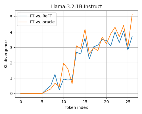
Here, we are taking generations on some prompts and comparing the average KL divergence between the fully fine-tuned model’s output probabilities and those of ReFT’s and the linearized oracle’s. The oracle often deviates further from the fine-tuned model than ReFT does, although not by much.

The best way around this would be to learn a low-rank, non-linear function as the map between the hidden states and the steering vectors. What better than a small autoencoder! Its output space would be constrained by the column space of the up-projection, so it will still be low-rank. This isn’t a new idea to steer post-skip-connection ([4] [5] for example), but the systematic justification presented here is: when steering block-by-block, post-block steering will be the most expressive.

At this point, it seemed like we understood what would likely work as a steering vector, so we moved away from using the oracle as the gold-standard to match and now worked on training these adapters end-to-end.

Post-Block Performance

Now we train these steering vectors without a guide. We add low-rank steering modules at the end of each block (similar in spirit to LoRA/PEFT), but applied to activations rather than weights. Based on the discussion above, we test two variants:

• Linear adapters: a simple low-rank adapters.
• Non-linear adapters: a down-projection, followed by a nonlinearity, then an up-projection (essentially a tiny autoencoder).

The nonlinear version is motivated by our earlier observation (and by [4] and [5]) that the map from hidden states to steering vectors may itself be nonlinear, while still being largely confined to a low-rank subspace.

Here are the results we’re currently seeing for 1B-parameter models:

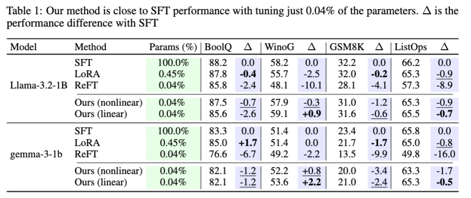
For a fair comparison, we match the parameter counts of our adapters to the baselines.

• For ReFT, we use rank-8 adapters for both ReFT and our method.
• For LoFIT, we train fixed vectors (rather than adapters) per layer.
• For JoLA, we train rank-1 adapters.

Across both Llama-1B and Gemma-1B, the trend is consistent: simply moving the steering location to post-block leads to a substantial boost in performance. Under identical parameter budgets, our linear post-block steering outperforms ReFT, and our fixed-vector and rank-1 variants outperform LoFIT and JoLA respectively.

In a few cases, linear steering even outperforms LoRA (learning an adapter on every Linear module) with the same rank, and occasionally out-performs SFT using full rank! This shows there are situations where steering is a better choice than finetuning.

What is surprising about these results is that linear steering is performing better than non-linear steering. Non-linear steering is not necessarily more expressive than linear steering (with the same rank), and for these tasks, it seems to be that the steering really is linear-like, validating the choice in ReFT. In this situation, it would be better to let the steering have more rank as a pure linear model rather than with some non-linearity messing with this structure.

Now compare this to some larger, 4B-parameter models:

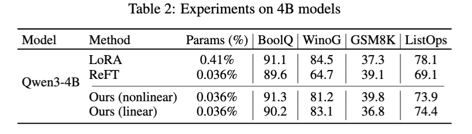
The behavior is different! Now, non-linear steering typically performs better than linear steering (except notably in Winogrande). This shift is likely due to optimization effects of the different scales of model tested here. At the larger scale, the loss function typically ends up being smoother/flatter than smaller scale models. This could mean the larger models can learn the more-expressive non-linear adapter over the easier-to-learn linear adapter.

Additionally, this shift could mean something more fundamental to the best adapters as well. If the adapter is well-suited as a linear adapter with the correct rank, the non-linear adapter would have to work around its non-linearity with something like large scale parameters to match the linear adapter. So, it’s possible that the smaller models need a small-rank linear adapter while the larger models need a large-rank non-linear adapter, but this is left to future work.

Theory

Post-block is better than Post-MLP

Now that we’ve seen how there is a clear difference between post-MLP and post-block steering, we now should ask why is there such a difference. What makes post-block steering better than post-MLP?

This difference, already highlighted, is that a post-block steer can depend on outputs of the attention layer without passing through the GLU. To gain some simple intuition, let’s take a 1-layer model, made of one Attention layer and one GLU:

where $x$ is the input of the model.

The two steerings we will be comparing are a post-MLP steer, that only depends on the outputs of the GLU, and a post-block steer, which steers the model after the skip-connection is added back into the model (which for this model, will just be another steer at the very end that depends on the original model outputs). Let’s remind ourselves of the structure of the GLU/MLP:

Consider the (fairly extreme) case where $W_d = 0$. In this situation, the GLU will be identically 0, so any input-dependent steering $\Delta y_{MLP}$ will be a fixed vector. Compare this to the post-block steering which can still depend on $h + \mathrm{Attn}(h)$. This also will extend to cases where $W_d$ is not full-rank, where the output of the steering cannot depend on the directions in the null-space, since the only contributions of a pre-MLP steer in the directions perpendicular to $\text{col}(W_d)$ will be a fixed-vector, while post-MLP steering does not have this restriction.

This tells us:

There are some situations that post-MLP steering does not perform well while post-block steering does.

Is it the case that post-block steering always can do what post-MLP steering can do? Unfortunately, no, not always. After adding back the skip-connection, it isn’t necessarily true that this is invertible so that the skip-connection and GLU terms can be distinguished; their subspaces might overlap with each other. In the situation when this isn’t true, we can match post-MLP steering perfectly.

To gain some intuition, let’s restrict ourselves to the linear case, where post-MLP steering is a steering in the style of ReFT. Now, to assure invertibility, assume that the subspace spanned by the skip-connection and the subspace spanned by the MLP outputs have trivial intersection. That is to say that there is a projection map $P$ such that

At this point, the equivalence is easy to see. If $A$ is the rank-$r$ linear projector for post-MLP steering, then $\Delta h(h) = A P h$ as a post-block steer will match the post-MLP steering perfectly. It will also be rank-$r$ since $AP$ is a rank-$r$ (or less) matrix.

Of course, this setting where these two vector spaces are completely separate is a bit extreme. Steering might need to be done in the same direction as the steered vector. At this point, some probability needs to be involved since any projection will no longer be perfect. However, we save this for the paper.

Error Control

One last thing to mention is that, since we have an oracle at each layer, it’s now possible to measure how similar we are to that oracle. This is, of course, assuming that we have access to the fine-tuned model we want to mimic. Soon we will remove this and move towards a more oracle-free understanding, but for the moment, assume we have access to this oracle. We also now have fine-grained control about errors and how they grow through the model! At each layer, it’s possible to develop an approximate steering vector $\Delta h’$ to match the oracle $\Delta h_{\mathrm{oracle}}$ closely enough that no layer has an error between them of more than some $\epsilon$.

Importantly, this gives us knowledge of how complex our adapters need to be. For example, if our update is nearly linear, we can take enough rank $r$ so that the approximation is within $\epsilon$ to ensure that that error does not grow out of control through the model.

The exact form of this required control is beyond the scope of this blog. However, there are a few key insights.

• The layer-norms help control the error significantly since in most models, their vector-wise standard deviation is somewhat large.
• Differences in hidden-states are amplified by the 2-norms of the matrices of each layer times $\sqrt{n}$, where $n$ is the representation dimension. The difference in 2-norm between the matrices ends up with a factor of $n$ instead, so it is more important that steering is more expressive on layers where the difference in matrices is larger (unsurprisingly so).

We plan to further improve these bounds with nicer assumptions based on the behavior of real models soon!

Note:: The model we analyze in this theory section is a drastically simplified stand-in for a real block, but the same geometry: post-block can see both Attn and GLU, post-MLP only sees GLU, persists in deeper models.

Where this leaves us

If you’ve made it this far—kudos! That’s pretty much all we have to say (for now, wink). To conclude, here are some highlights of everything we unpacked:

• Pre-MLP vs. Post-MLP: They behave very differently, and post-MLP generally does a better job matching MLP weight updates.
• But Post-Block is generally better than Post-MLP. Steering the residual stream, not individual module outputs, is the real sweet spot.
• With only 0.04% trainable parameters (compared to LoRA’s 0.45% using the same rank), our method at this post-block location gets remarkably close to SFT, which updates all parameters.

Where do we go from here?

Lowering the number of trainable parameters is more than an efficiency win. It buys us compute headroom for adapting larger models, running more expensive algorithms like RL, and we can do all of this within realistic compute budgets.

Because our framework reasons about steering and weight updates in their most general form (arbitrary $\Delta h$ and arbitrary $\Delta W$), there’s nothing stopping those updates from being learned by far more expensive methods (e.g., GRPO or other RL-style objectives). So the natural next step is clear: test whether our steering can plug into these stronger algorithms and deliver the same performance with a fraction of the trainable parameters.

And now that we know it’s possible to learn nearly as well in activation space as we can in weight space in even more setting than ReFT originally could, an even more ambitious idea opens up:

What happens if we optimize in both spaces together?

Perhaps, jointly optimizing them might help us break past the limitations or local minima that each space hits on its own?

Stay tuned to find out!

🧪 Want to try it yourself?

We’ve packaged everything — activation adapters, post-block steering layers, training scripts — into a clean, lightweight library.

👉 **Try our code on GitHub** 🐙

References

[1] Wu, Z., Arora, A., Wang, Z., Geiger, A., Jurafsky, D., Manning, C., & Potts, C. (2024). ReFT: Representation Finetuning for Language Models.

[2] Fangcong Yin, Xi Ye, & Greg Durrett (2024). LoFiT: Localized finetuning on LLM Representations. In The Thirty-eighth Annual Conference on Neural Information Processing Systems.

[3] Lai, W., Fraser, A., & Titov, I. (2025). Joint Localization and Activation Editing for Low-Resource finetuning. arXiv preprint arXiv:2502.01179.

[4] Houlsby, N., Giurgiu, A., Jastrzebski, S., Morrone, B., De Laroussilhe, Q., Gesmundo, A., … & Gelly, S. (2019). Parameter-efficient transfer learning for NLP. In International conference on machine learning.

[5] Tomanek, K., Zayats, V., Padfield, D., Vaillancourt, K., & Biadsy, F. (2021). Residual adapters for parameter-efficient ASR adaptation to atypical and accented speech. In Proceedings of the 2021 Conference on Empirical Methods in Natural Language Processing.

Appendix

Implementation details:

For all methods, we sweep across 5 learning rates and keep other hyperparameters constant (batch size, scheduler, warmup ratio, weight decay). We keep the same learning rate sweep space for ours, ReFT, JoLA, and LoFIT, and slightly shift to smaller values for SFT and LoRA (since they train substantially more parameters).

The ReFT paper also treats the tokens to steer as a hyperparameter. After selecting the best learning rate, we sweep over two locations: the last prompt token (the default value) and (prefix+7, suffix+7) (the best configuration reported for GSM8K). Our method does not require this sweep, it intervenes at all token positions (both prompt and generated).

• SFT sweep values: [5e-6, 1e-5, 2e-5, 5e-5, 1e-4]
• LoRA sweep values: [5e-5, 1e-4, 3e-4, 7e-4, 1.5e-3]
• Activation steering methods sweep values: [5e-4, 1e-3, 2e-3, 3e-3, 5e-3]