One exciting aspect of large pretrained ‘foundation’ models is that it is easy to obtain multiple observations by repeatedly querying. The most straightforward example is to obtain multiple answers to a question by varying the prompt, as shown below. These outputs could be noisy and naturally, we’d like to aggregate these outputs in such a way that we obtain a better estimate of the ground truth than any single answer on its own. Ideally, this aggregation should

• Take into account that some estimated objects are closer to the ground truth than others, i.e., are more accurate, and upweight these,
• Be fully unsupervised—so that we have no access to the ground truth and can be fully zero-shot,
• Work with structured objects—not just model outputs, but chains, trees, and other intermediate structures used in techniques like chain-of-thought (CoT) prompting and other reasoning approaches.

In this post we discuss a simple way to do this based on one of our NeurIPS ‘22 papers. The core principle is a (very general) form of the weak supervision algorithms that we’ve been playing with for several years. For binary outputs, this idea has already been successfully used in our Ask Me Anything prompting strategy. Here, we focus on lifting this to the richer structures needed for CoT and other techniques.

Warning: our discussion will get a bit technical—but we promise it will be fun! In fact we’ll get to connect to a ton of different fields, including graphical models, unsupervised learning, embeddings and non-Euclidean geometry, tensor algorithms, and more!

First, a roadmap for this post. We will

• Cover some well-trodden ground on the fundamentals of simple aggregation. We’ll model noisy observations of binary objects and describe a very simple approach to learn how accurate the observations are, without ground truth. This part will also serve as a short introduction to weak supervision.
• Apply a powerful algorithm based on tensor decomposition—enabling us to relax our modeling assumptions for aggregation, in the hope we can aggregate complex objects.
• Figure out how to scale it up to rich structures by operating on a very special type of embedding, called pseudo-Euclidean.
• Show on a toy example how this can help us improve CoT beyond simple approaches like majority vote.

Let’s dive in!

Aggregation Fundamentals

Let’s take the example in the figure above. We are performing a basic email classification task, where we want to categorize each message as spam or not spam. We repeatedly query the model by varying the prompt, obtaining a number of observations for each email.

We’ll refer to each prompting approach as an object source (OS). These sources are just estimates of the ground truth answer for whatever task we’re interested in. What can we do with these? First, let’s collect the outputs. These are arranged in a matrix as shown in figure below. The instances (examples) are the emails. Of course, the column for the ground truth label $Y$ is just a placeholder since we don’t get to see it.

After observing the outputs of the sources, the goal of aggregation is to estimate the ground truth object—and hopefully more accurately than any single source by itself! A naive but reasonable first-cut way to aggregate is to take the majority vote of the outputs for each point. This approach will work well when the OSs are independent and have similar qualities. However, some OSs could be more accurate and some more noisy. They might also be correlated. This can make majority vote less effective. Imagine, for example, that one source is right 95% of the time, while the others are right only 51% of the time. Clearly aggregation will help, but we’d like to dramatically upweight the accurate source.

How can we model these possibilities? Weak supervision approaches often model the distribution of the unobserved ground truth $Y$ and source outputs $\lambda_1, \ldots \lambda_m$ as a probabilistic graphical model with parameters $\theta$, for example the Ising model:

What does this do for us? First, we can now think of learning the accuracies and correlations described above as learning the parameters of this model. These are the $\theta$’s, also known as canonical parameters in the PGM literature. Note that unlike conventional learning for graphical models, we have a latent variable problem, as we do not observe $Y$. If we have learned these parameters, we can rely on the estimated model to perform aggregations. The resulting pipeline looks like:

The $\theta$ parameters above encode how accurate each of the OSes are, with a large $\theta_i$ indicating that the $i$th noisy estimate frequently agrees with $Y$, the ground truth. How do we estimate these? We’ll need a few technical pieces from the graphical model literature. It turns out that we need only estimate the mean parameters—terms like $\mathbb{E}[\lambda_i Y]$ and $\mathbb{E}[\lambda_i \lambda_j]$! Note that the correlation terms $\mathbb{E}[\lambda_i \lambda_j]$ do not involve $Y$ — so that as long as we know the structure (the edge set E), the rest is easy, since these terms are observed.

How about the accuracy parameters i.e., the correlations between $\lambda_i$ and $Y$ ? This is challenging as we don’t get to see any ground truth! There are classical methods like EM (Expectation-Maximization) and variants such as Dawid-Skene that could be applied. However, these approaches are prone to converging to local optima and sometimes perform poorly. A simple and elegant approach, Flying Squid, based on the Method of Moments, to the rescue! The key idea is based on the observation that for any three conditionally independent sources, $\lambda_1,\lambda_2,\lambda_3$ the second order moments with binary labels can be written as,

This system of three equations can be solved directly for $\mathbb{E}[\lambda_i Y]$ without observing $Y$, as follows. \(|\mathbb{E}[\lambda_1 Y]| = \sqrt{\frac{\mathbb{E}[\lambda_1\lambda_2] \mathbb{E}[\lambda_3\lambda_1] }{\mathbb{E}[\lambda_2\lambda_3]}}, |\mathbb{E}[\lambda_2 Y] |= \sqrt{\frac{\mathbb{E}[\lambda_1\lambda_2] \mathbb{E}[\lambda_2\lambda_3] }{\mathbb{E}[\lambda_3\lambda_1]}}, |\mathbb{E}[\lambda_3 Y]| = \sqrt{\frac{\mathbb{E}[\lambda_2\lambda_3] \mathbb{E}[\lambda_3\lambda_1] }{\mathbb{E}[\lambda_1\lambda_2]}}\) This analytical solution is easy to obtain for the binary classification setting. All that is left is to figure out the signs of the above, in order to break symmetry. As long as our sources are better than random on average, this can be done.

What does knowing these accuracies buy us? It turns out that we can use them to do weighted aggregation, or, more concretely given our model, to compute a posterior probability \(P_{\hat{\theta}}(Y \vert \lambda_1, \ldots, \lambda_m)\).

This basic idea can also be extended easily to multi-class settings by solving multiple one vs. rest binary classification problems. This method has nice theoretical guarantees and works well for classification settings especially when the number of classes is small—and when the model has special kinds of symmetry. More details about FlyingSquid can be found in the blog post and paper. Try it!

Aggregation with Tensor Decompositions

As we saw, the main challenge in WS is to estimate the accuracies $\theta_i$ of the object sources without having access to the ground truth object. While approaches like FlyingSquid are simple and efficient, they make some strong assumptions. If we want to handle outputs that have high-cardinality or special structure (e.g. parse trees, rankings, math expressions etc.), we may need a more powerful tool. Tensor decompositions are a great candidate for this—having already been used for learning many kinds of mixtures. Before we proceed, let’s see how we can adapt this class of algorithms to our aggregation setting.

We’ll start with some quick background on classical multi-view mixture model learning. Our first task is to understand if it is suitable for aggregating more complicated foundation model objects. As a first step, we ask if it works on par with existing methods for simple settings like binary classification? If so, does it directly scale up to more challenging objects, such as those that take on many possible values?

We’ll see that tensor methods are competitive for simple cases, but that this approach doesn’t scale well when the objects live in higher-cardinality spaces with structure. To make it possible to use tensor decomposition approaches for such scenarios, we’ll have to make some careful adjustments.

Multi-View Mixtures and Tensor Decomposition

We can think of source outputs as observations from a multi-view mixture model i.e., each source $\lambda_a$ is a view of the true object $Y$. In a multi-view mixture model, multiple views \(\{\lambda_{a}\}_{a=1}^m\) of a latent variable $Y$ are observed. These views are independent when conditioned on $Y$. i.e. $\lambda_{a}\vert Y=y$ is conditionally independent of $\lambda_{b}\vert Y=y$ for all $a,b$. This mixture model is depicted as a graphical model in the below figure.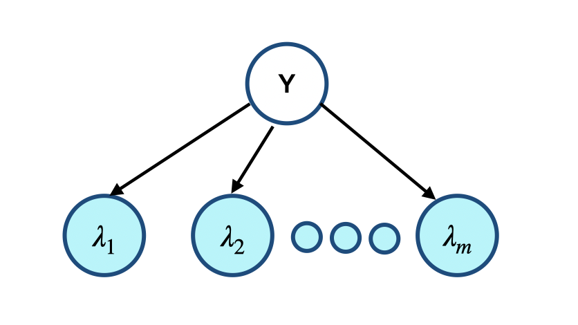

Now, suppose we have a cardinality $k$ problem (the true object $Y$ takes $k$ values). We use one-hot vector representations of the objects ( denoted in bold-face ). Let \(\mathbb{E}[{\boldsymbol{\lambda}}_a|Y=y] = {\boldsymbol{\mu}}_{ay}\) denote the mean of \(\boldsymbol{\lambda}_a\) conditioned on the true object $y$ (for all $a$ and $y$). Then it is easy to see the following for the tensor product (third order moment) of any three conditionally independent ${\boldsymbol{\lambda}}_a,{\boldsymbol{\lambda}}_b,{\boldsymbol{\lambda}}_c$,

i.e. $\bf{T}$ can be written as a sum of $k$ rank-1 tensors. Here $w_y \in [0,1]$ are the prior probabilities of label $Y=y$. Note that we do not know the true distribution of $\lambda,y$. Instead we have $n$ i.i.d. observations \(\{ {\boldsymbol{\lambda}}_{a,i}\}_{a\in[m],i\in[n]}\). Using these we can produce an empirical estimate of $\bf{T}$:

Suppose \(\tilde{\bf{T}} = \sum_{y\in[k]} \hat{w}_y \hat{\boldsymbol{\mu}}_{a,y}\otimes \hat{\boldsymbol{\mu}}_{b,y} \otimes\hat{\boldsymbol{\mu}}_{c,y}\) is a rank-k factorization of the empirical tensor $\hat{\bf{T}}$. If $\hat{\bf{T}}$ is a good approximation of the true tensor ${\bf{T}}$ and $\tilde{\bf{T}}$ is a good approximation of $\hat{\bf{T}}$ then we have that \(\hat{\boldsymbol{\mu}}_{a,y}\) is good approximation of the true mean parameters ${\boldsymbol{\mu}}_{a,y}$. This idea is developed in the fantastic Anandkumar et al. 2012, 2014 and lots of follow-up work.

Using the estimates $\hat{\boldsymbol{\mu}}_{a,y}$ we obtain estimates of our canonical $\theta$ parameters, and so we’ll have the accuracies, just as with FlyingSquid or other weak supervision methods. We’ll call this procedure the tensor aggregation model.

Tensor Aggregation Model is Competitive in Basic Settings… But We Need More

The big question—how well does this work? We run a simple experiment on simulated sources to show that this method is competitive. For this we simulate three object sources outputting multiclass values with $\theta=[4,0.5,0.5]$. We run tensor aggregation on the 1-hot encodings of the outputs and compare the accuracy of the aggregated object against FlyingSquid and majority vote baselines. The results are shown in figure below (averaged over 100 trials). Tensor aggregation offers competitive performance but due to the use of 1-hot encodings—leading to high dimensionality—its performance also degrades when we increase the cardinality of the object space.

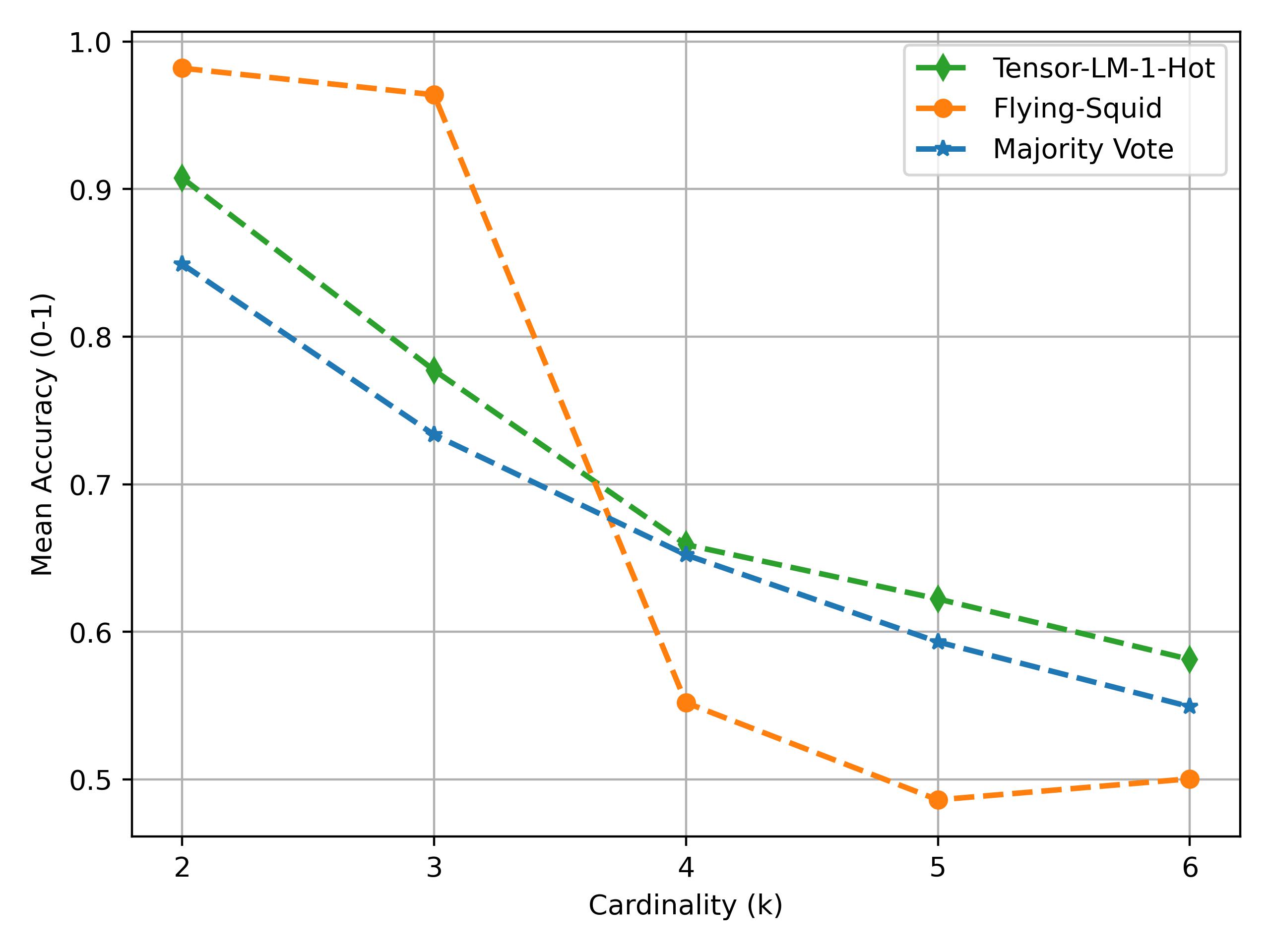
Note that we used the simplest one-versus-all approach to multiclass FlyingSquid. There are much more powerful variants that would likely out-compete (as is the case for binary)—but for simplicity, we won’t include all of these.

Overall, the tensor method is encouraging and we’re motivated to apply it beyond simple classification settings. How do we scale up to such settings?

Interlude: Aggregation Beyond Categorical Objects

As we alluded to, many foundation models will require aggregating items more diverse than just a multiclass label. Even more generally, we’ll often want to aggregate a huge range of object types. We’ve thought about how to do this with semantic dependency parse trees, classes of objects having hierarchal structure, continuous or manifold-valued objects for regressions, and more. We can often think of the spaces these objects live in as metric spaces—since they have natural distance functions. Here we’ll discuss the finite metric space case, but we have lots of ideas about how to extend it to infinite cardinality spaces. Our approach consists of two high level steps:

• First we learn isometric representations of the objects using a classical—but surprisingly little-known—tool called pseudo-Euclidean embeddings (PSE),
• We then adapt the tensor aggregation procedure to work with PSE embeddings.

As we shall see, both of these steps are critical. We show a full pipeline below.

Distortion-Free Embeddings

Now that our objects of interest live in metric spaces, our new goal is to aggregate them into something close to the ground truth. For example, suppose the distance metric is $d$. We’d like to again aggregate $\lambda_a, \lambda_b, \lambda_c$. Ideally we’d like to get an output $\hat{y}$ so that $\mathbb{E}[d(\hat{y}, y)]$ is small. Once again, we’d need to account for accuracies—which are now average distances like $\mathbb{E}[d(\lambda_a, y)]$.

Working directly with discrete metric spaces is challenging—we can’t use our favorite off-the-shelf optimization approaches. To make life easy we’ll do the usual: work with low-dimensional vector space representations. If we can do this, we’ll be set: we’ll get away with using tensor aggregation without needing to scale it up to high dimensions, where we could get hurt by noise, as we saw earlier.

The key is to have these low-dimensional representations preserve distances, since otherwise we can’t hope to perform a reasonable aggregation. That is, if our embeddings of objects distort these distances, our aggregation might end up with a distant output $\mathbb{E}[d(\lambda_a, y)]$. Learning faithful embeddings has been a very active area of research over several decades. Here we are particularly interested in learning isometric—perfectly distance-preserving—embeddings.

In general, such isometric embeddings might not exist in the conventional case of vector space embeddings. Instead, we use Pseudo-Euclidean Embeddings (PSE). These are a generalization of classical Multi-Dimensional Scaling(MDS). The main benefit of PSE over MDS is that it can isometrically embed metric spaces that cannot be isometrically embeddable in Euclidean space. The main drawback, as we shall see, is that pseudo-spaces are weird!

We’ll discuss PSE more technically below, but first let’s understand its utility. As an example, take our metric spaces to be graphs, where the distance is the smallest number of hops between nodes. Two examples of graphs are shown below. We learn their node embeddings using MDS and PSE. MDS gives low dimensional representations but cannot produce isometric embeddings for general metric spaces. Note that MDS (blue line) never reaches zero—but with just three-dimensional embeddings, PSE does! For a more complex graph, the tree to the right, we see the same effect. Adding dimensions helps MDS a bit, but fails to produce isometric embeddings, while PSE succeeds again (red line drops to $10^{-14}$).

How do these pseudo-Euclidean spaces work? Basically, their metrics are no longer induced by p.s.d. inner-products, so that we can have distinct points still have distance 0. This is behavior that is often challenging to deal with geometrically, but for our purposes, works fine.

Let’s see some technical details: a vector ${\bf{u}}$ in a pseudo-Euclidean space $\mathbb{R}^{d^+,d^-}$ has two parts: ${\bf{u}}^+ \in \mathbb{R}^{d^+}$ and ${\bf{u}}^- \in \mathbb{R}^{d^-}$. The dot product and the squared distance between any two vectors ${\bf{u}},{\bf{v}}$ are $\langle {\bf{u}}, {\bf{v}}\rangle_{\phi} = \langle {\bf{u}}^+,{\bf{v}}^+ \rangle - \langle {\bf{u}}^-,{\bf{v}}^- \rangle$ and $d^2_{\phi}({\bf{u}},{\bf{v}}) = \lVert{\bf{u}}^{+}-{\bf{v}}^{+}\rVert_2^2 - \lVert {\bf{u}}^{-}-{\bf{v}}^{-}\rVert_2^2$. These properties enable isometric embeddings: the distance can be decomposed into two components that are individually induced from p.s.d. inner products—and can thus be embedded via MDS. Indeed, pseudo-Euclidean embeddings effectively run MDS for each component. To recover the original distance, we obtain $\lVert {\bf{u}}^{+}-{\bf{v}}^{+}\rVert_2^2$ and $\lVert{\bf{u}}^{-}-{\bf{v}}^{-}\rVert_2^2$ and subtract. More details on these embeddings can be found in a classic treatise.

Upgrading Structured Aggregation with PSE

Armed with the powerful PSE technique, we first obtain isometric representations of the objects in a PSE space and solve the parameter estimation problem using tensor decomposition. The original tensor decomposition algorithm was designed for Euclidean vectors so we cannot apply it off-the-shelf for PSE points. We overcome this issue by using the fact that the two parts of any vector in PSE are individually in Euclidean spaces $\mathbb{R}^{d^+},\mathbb{R}^{d-}$ . This allows us to treat the positive and negative components \({\boldsymbol{\lambda}}_{a}^+ \in \mathbb{R}^{d^+}\) and \({\boldsymbol{\lambda}}_{a}^{-} \in \mathbb{R}^{d^-}\) of our pseudo-Euclidean embedding as separate multi-view mixtures. We apply tensor decomposition on them separately, which gives us mean parameters \(\hat{\boldsymbol{\mu}}^+_{a,y}\) and \(\hat{\boldsymbol{\mu}}^-_{a,y}\) for each $a,y$. Using these we obtain our estimates of the canonical parameters \(\hat{\bf{\theta}}\).

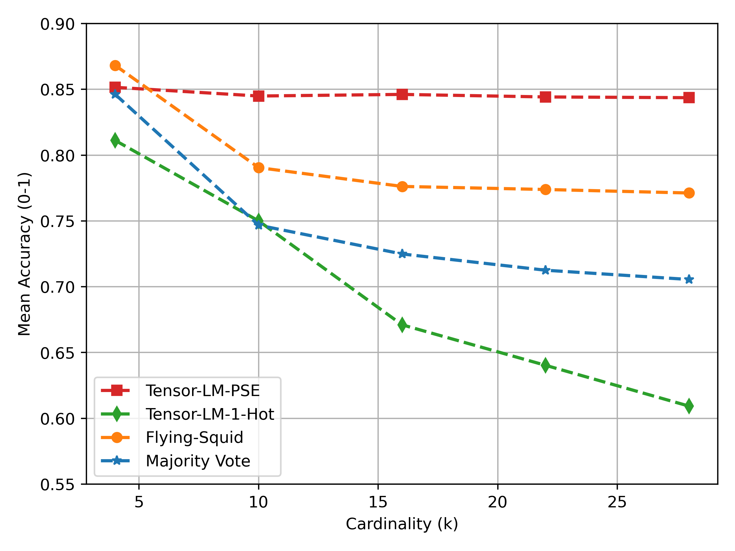With this adaptation, we retain the nice theoretical guarantees of tensor decomposition for parameter recovery while working with any finite metric space. We can also see the benefit of our approach on a simple synthetic data experiment on the tree metric we saw earlier. In this experiment, we simulate three sources on the tree metric with three branches with $b$ number of nodes in each branch. We use $\theta=[4,0.5,0.5]$ i.e. first source is highly accurate and the other two are somewhat noisy. We run two variations of our method one with PSE embeddings and the other with 1-hot embeddings of the labels. We keep the number of samples $n=1000$ fixed and vary the number nodes $b$ to increase the cardinality of the label space. The results can be seen in figure below.

As expected, using PSE embeddings we can achieve much better accuracy of the aggregated objects and unlike other methods this performance does not degrade with higher cardinality, as this metric space is isometrically embeddable in 3-dimensional PSE space.

Putting It Together: Aggregating Chain-of-Thought

This aggregation approach is quite general and can be applied in any setting where we can obtain multiple noisy observations of a ground truth object living in a discrete metric space.

We’ll show off its potential in a toy CoT example. We consider in-context learning for language models. The in-context examples typically consist of paired input and output data, which effectively guide LLMs in comprehending the task at hand and generating accurate predictions. Recent advancements in this area have shed light on the effectiveness of prompts that incorporate explicit steps known as Chain of Thoughts (CoT). These step-by-step instructions facilitate LLMs in making precise predictions while providing detailed reasoning steps. Building upon this concept, more nuanced variations such as Tree of Thought (ToT) and Graph of Thought (GoT) have emerged. These expanded frameworks have demonstrated impressive efficacy when tackling complex reasoning problems with LLMs.

While highly effective, they require access to high quality explanations which can be a bottleneck in broad applicability of these methods. Nevertheless, one can always come up with many self-obtained, or heuristic, or otherwise inexpensive sources that can provide potentially noisy reasoning steps. How can we use these to construct accurate chains or trees or graphs of thoughts?

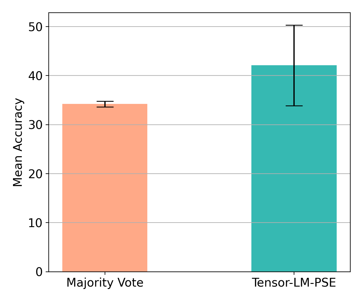
Indeed, we can use our aggregation approach. As an illustration, we consider the Game of 24, a complex reasoning puzzle with 4 numbers from 1 to 13 as input. The expected output is an expression using the given numbers and basic arithmetic operations (+,-,x,/) so that the expression evaluates to 24. Note that this task can be easily solved by enumerating all possible expressions and selecting the ones that evaluate to 24. However, we are interested in solving this task using LLMs by providing it some in-context examples. Here the CoT steps could be an expression broken down into multiple steps. We use the same 1362 puzzles as in Tree of Thought paper and simulate 3 sources with different noise levels ( $\theta= [5,0.6,0.5]$ ) that can provide noisy expressions (CoTs). We then apply our aggregation procedure (i.e., PSE + tensor decomposition() to recover the true expressions and evaluate the recovered expressions for the correctness. We run this procedure 10 times with different random seeds and report the mean accuracies in the above bar chart. We can clearly see that our method based on tensor decompositions output performs majority vote.

Although on a small-scale toy problem, these findings are quite exciting and demonstrate the potential of weak supervision for aggregating foundation model objects, such as in CoT, ToT, GoT or other forms of reasoning.

Takeaways and Future Work

1. Weak supervision techniques are awesome at aggregating noisy sources to estimate ground-truth objects.
2. Building on top of classical tools – tensor decomposition and pseudo-Euclidean embeddings, we provide an aggregation method that works well for combining objects living in finite metric spaces.
3. Lots to explore! We used isometric embeddings—can we get away with even fewer dimensions by allowing these to be slightly distorted? Can we scale up this procedure to use very large reasoning chains, trees, and other structures? Can we smoothly integrate this procedure into foundation model inference pipelines?

We hope you enjoyed our post! Please check out our paper, and our code!