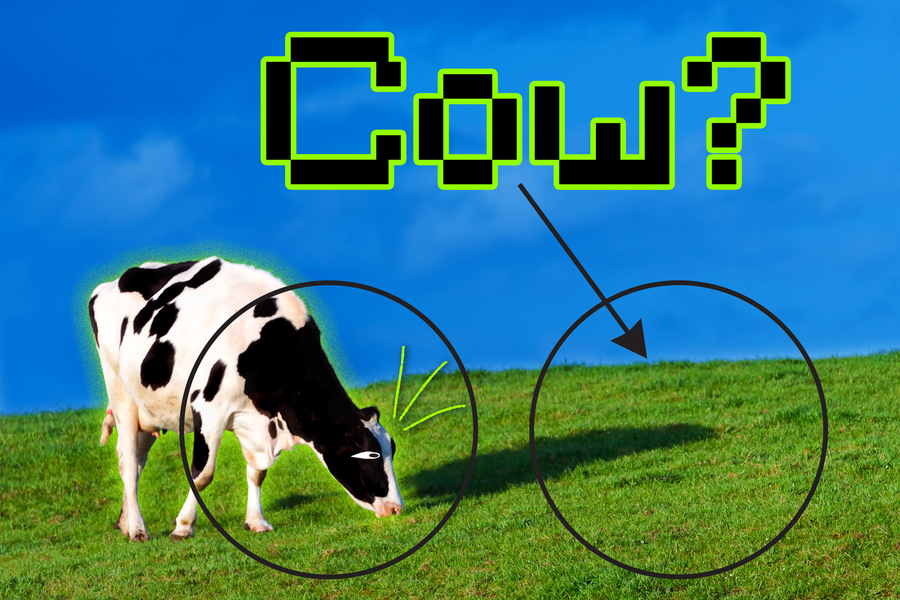
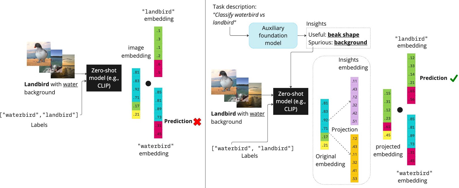
Large pre-trained multi-modal models (e.g., OpenAI’s CLIP) are strong zero-shot predictors–achieving 77.9% zero-shot accuracy on CIFAR100. Now practitioners can use them out of the box for downstream prediction tasks without fine-tuning. Unfortunately, such models can adopt biases or unwanted correlations from their large-scale training data – making their predictions less reliable on samples that break in-distribution correlation. For instance, they might associate ‘cow’ with ‘green’; because cow images are mostly depicted with pastures in the training data. But then, making wrong predictions on images of, let’s say, cows on the beach.

Robustness against these spurious correlations have been widely studied in the literature. Sagawa et al., 2019 brings into attention the discrepancy between model performance on data slices that conform to training data biases vs. those that break the correlations. A plethora of methods similar to Arjovsky et al., 2019 tackle this during training stage, which render them less practical for large pre-trained architectures. Zhang & Ré, 2022 demonstrated the performance discrepancy between different data slices is also apparent in pre-trained models, and propose a lightweight adapter training approach. Yang et al., 2023 introduces a spurious correlation aware fine-tuning approach. However, some might argue that fine-tuning breaks some promise of large pre-trained models – their capacity to be used out of the box.

In this post we describe Roboshot: an approach to robustify pre-trained models and steering them away from these biases/correlations. What’s more? RoboShot does this without additional data and fine-tuning! The core of our idea is inspired by embedding debiasing literature, which seeks to remove subspaces that contain predefined harmful or unwanted concepts. However, here we do not seek to produce fully-invariant embeddings; our goal is simply to improve pre-trained model robustness at low or zero cost.

Zero-shot inference and modeling

Before diving in, let’s first discuss and formulate the zero-shot inference setup. Similar to Dalvi et al., 2022 we think of pre-trained models embedding space as spanning unknown concepts ${z_1, z_2, \ldots, z_k}$, and a pre-trained embedding $x$ is a mixture of concepts $\Sigma_i \gamma_i z_i$, where $\gamma_i \geq 0$ are weights.

Now, given $x$, $c^0=\sum_i \beta_{i,0} z_i$ (embedding of the first class), and $c^1=\sum_i \beta_{i,1} z_i$ (embedding of the second class) , its zero-shot prediction is made by

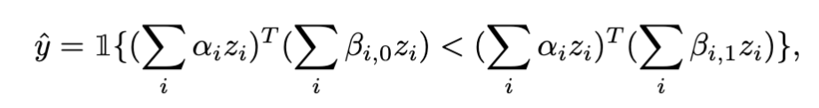
Prediction is made by taking the class with higher inner product with the datapoint’s embedding. The above equation describes binary classification, but it is straightforward to extend it to multi-class settings.

RoboShot assumes that input embedding mixture can be partitioned into three concept groups: harmful, helpful, and benign

For better illustration, we will start with a working example of a benchmark dataset: Watebirds. The task is to distinguish $y \in {\texttt{waterbird}, \texttt{landbird}}$. The training data contains unwanted correlations between waterbird and water background, and landbird with land background. For the sake of illustration, let’s assume that in the embedding space, $z_{water} = -z_{land}$ and $z_{waterbird} = -z_{landbird}$.

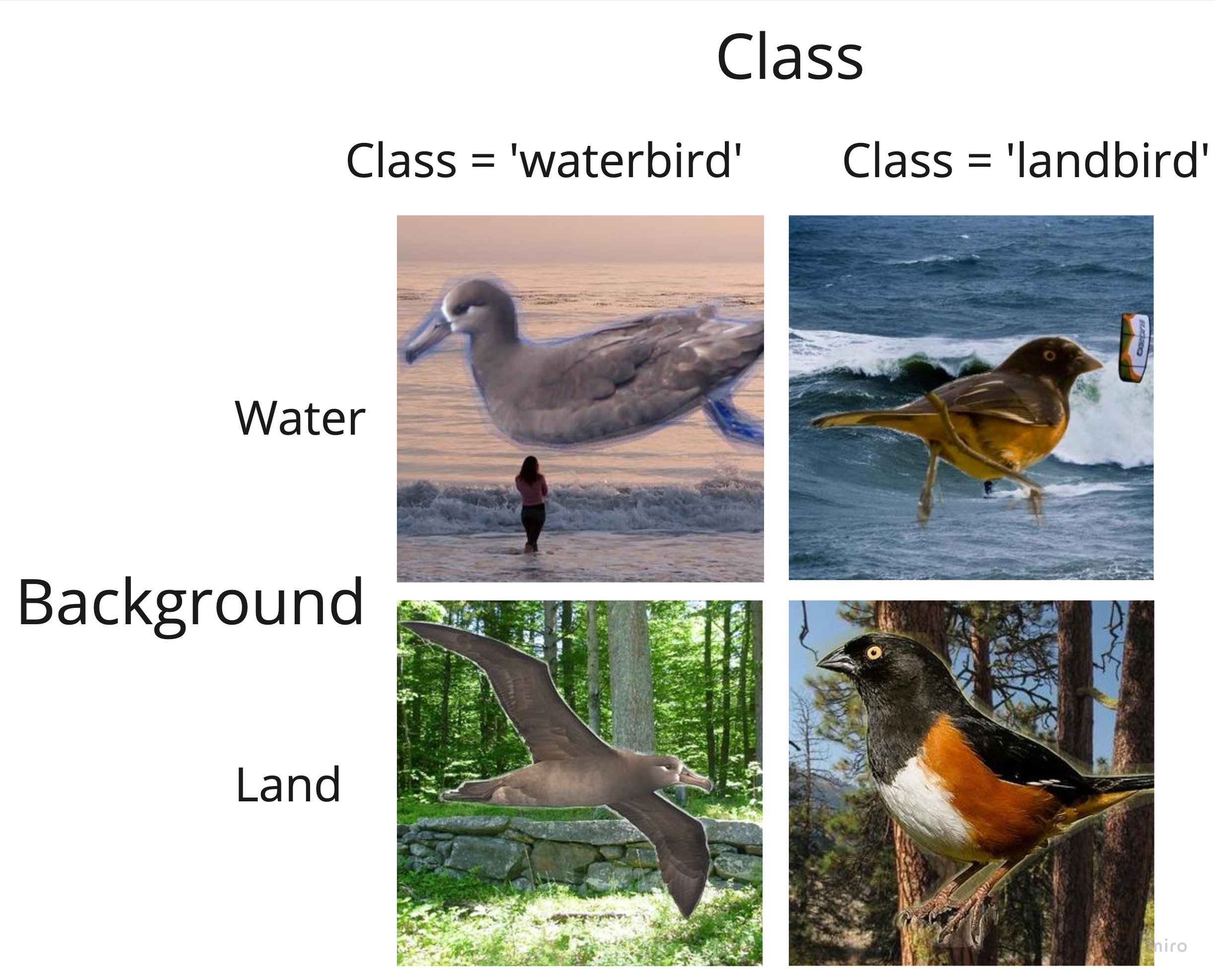
Let’s say we have a test image that does not follow the training correlations (e.g., landbird over water). In the embedding space, this might be $x=0.7z_{\texttt{water}}+ 0.3 z_{\texttt{landbird}}$

Our class embeddings might be $c^{\texttt{waterbird}}=0.4z_{\texttt{water}}+0.6z_{\texttt{waterbird}} \text{ and }c^{\texttt{landbird}}=0.4z_{\texttt{land}}+0.6z_{\texttt{landbird}}$

Our zero-shot prediction is then $x^T c^{\texttt{waterbird}}= 0.1 > x^T c^{\texttt{landbird}}= -0.1$

which gives us waterbird prediction and is incorrect.

In this example, we see how harmful components contained in $x$ cause wrong predictions. Now, let’s see how RoboShot avoids this by reducing harmful components in embeddings and boosting the helpful ones.

RoboShot

Suppose in $x$ we have ground truth harmful component $v^{\texttt{harmful}}$ and ground truth beneficial component $v^{\texttt{helpful}}$. Note that in reality, we do not have access to the $v^{\texttt{harmful}}$ and $v^{\texttt{helpful}}$ (in the next part of this blogpost, we will describe the proxy for this ground truth component). RoboShot reduces $v^{\texttt{harmful}}$’s effect on $x$ by classical vector rejection:

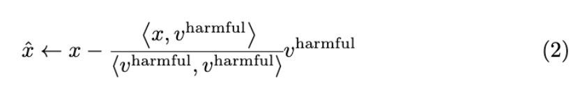
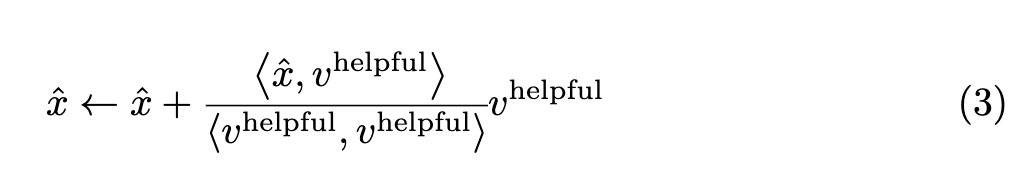
Intuitively, this procedure subtracts $v^{\texttt{harmful}}$’s component on $x$. Similarly, to increase $v_{\texttt{helpful}}$’s influence, we can add $v^{\texttt{helpful}}$’s component along $x$, such that:

Let’s try this on our example.

Suppose that we have a single harmful and helpful insight:

$v^{\texttt{harmful}}=0.9z_{\texttt{water}}+0.1z_{\texttt{landbird}} \quad \quad v^{\text{helpful}}=0.1z_{\texttt{water}}+0.9z_{\texttt{landbird}} $

First let’s reduce $v^{\texttt{harmful}}$’s effect by plugging it into equation 2, which results in $\hat{x} = -0.0244z_{\texttt{water}}+0.2195z_{\texttt{landbird}}$

Making zero shot prediction with $\hat{x}$, we have $x^T c^{\texttt{waterbird}}= -0.1415 < x^T c^{\texttt{landbird}}= 0.1415$

Which gives us the correct prediction: landbird

We have seen that removing a single component neutralizes the harmful component and now we have the correct prediction! Next, let’s see the effect of increasing $v^{\texttt{helpful}}$’s effect by plugging it into equation 3. This results in

$\hat{x} = -0.0006z_{\texttt{water}}+0.4337z_{\texttt{landbird}}$

This further increase the classification margin!.

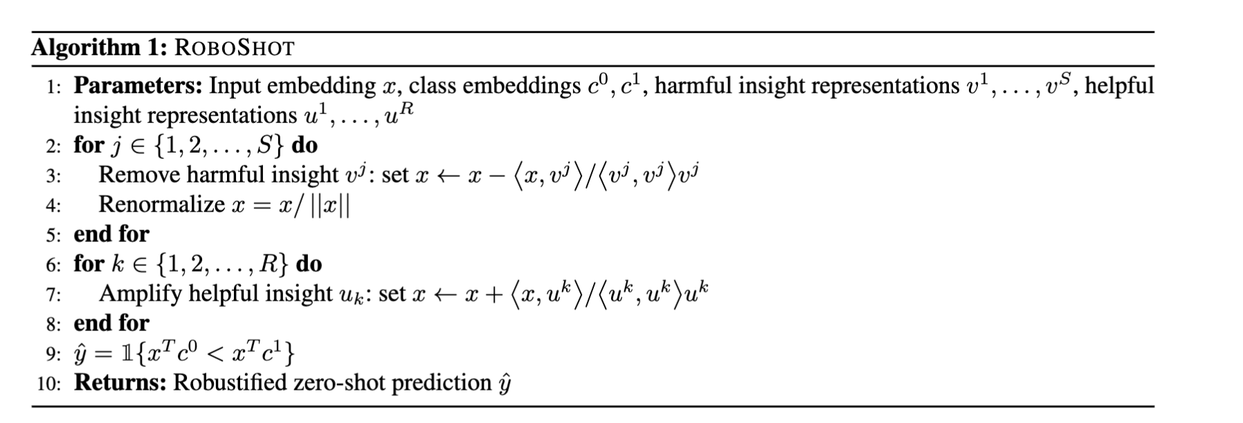
Algorithm 1 details the RoboShot algorithm. In real scenarios, we often have multiple helpful and harmful concepts (e.g., shape of beak, wing size, etc). We can simply do the vector rejection and addition iteratively (lines 2-5 and 6-8, respectively).

Using LLM to obtain proxy to $v^{\texttt{harmful}}$ and $v^{\texttt{helpful}}$

In real scenarios, how do we get access to $v^{\texttt{harmful}}$ and $v^{\texttt{helpful}}$? especially since in latent space, features are entangled with one another.

First let’s take a step back and think of $v^{\texttt{harmful}}$ and $v^{\texttt{helpful}}$ in the context of the task. For instance, in the Waterbirds dataset, the task is to distinguish between landbird and waterbird. Ideally, our predictions should be dependent only on the bird features (e.g., beak shape, wings size), and independent of confounding factors like backgrounds (i.e., land or water). If we can somehow isolate the background and bird components in the embedding space, set them as $v_{\texttt{harmful}}$ and $v_{\texttt{helpful}}$, and plug equations 2 and 3, we are golden. Wait, this is analogous to setting $v^{\texttt{harmful}}$ as the background features, and $v_{\texttt{helpful}}$ as the bird features! This way, we can think of $v^{\texttt{harmful}}$ and $v^{\texttt{helpful}}$ as a priors inherent to the task. Now, we have two remaining pieces to tie it all together: (i) how to obtain these insights without training, and (ii) how to translate them in latent space.

In RoboShot, we get the textual descriptions of harmful and helpful concepts by querying language models (LM) using only the task description. For example, in the Waterbirds dataset, we use the prompt “What are the biased/spurious differences between waterbirds and landbirds?”.

We translate the answers we get to $v^{\texttt{harmful}}$ , by using their embeddings. Let $s^1, s^2$ be the text insights obtained from the answer (e.g., {‘water background’ ‘land background’}). We obtain a spurious insight representation by taking the difference of their embedding:

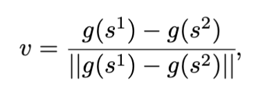
where $g$ is the text encoder of our model.

Similarly, to obtain proxy to $v^{\texttt{helpful}}$, we ask LMs “What are the true characteristics of waterbirds and landbirds?” and obtain e.g., {‘short beak’, ‘long beak’}. The remainder of the procedure is identical to the case of harmful components.

RoboShot in action

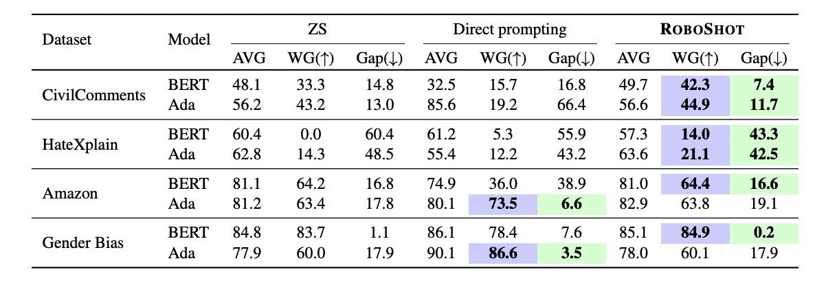
Thats it! With this cheap and finetuning free approach, now we can robustify our zero-shot models against unwanted correlations from training data. In the table below, we measure baseline and our performance in terms of average accuracy across all groups (AVG), worst-group accuracy (WG), and the gap between then (Gap). A model that is less influenced by unwanted correlations have high AVG and WG, and low Gap. We can see that Roboshot improves Vision-language model predictions across multiple spurious correlation and distribution shift benchmarks.

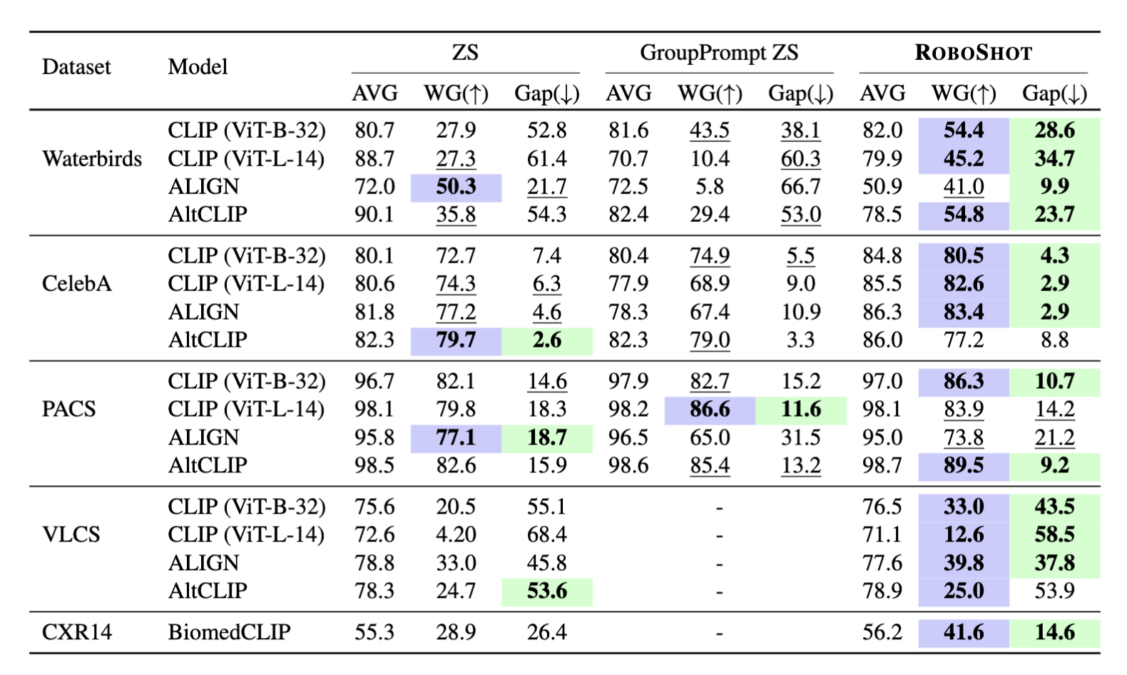
On language tasks, RoboShot also lifts weaker/older LMs performance to a level comparable to modern LLMs, and surpass direct prompting to BART-MNLI and ChatGPT on several datasets.

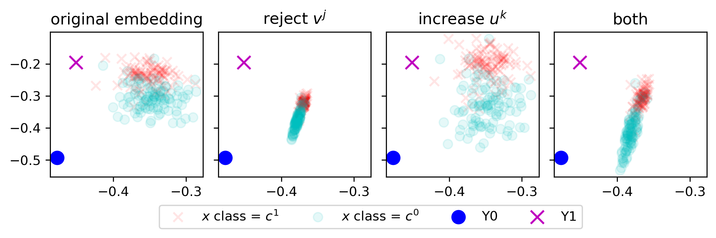
Below, we illustrate the effect of rejecting $v^{\texttt{harmful}}$, increasing $v^{\texttt{helpful}}$, and doing both in the following image. Rejecting $v^{\texttt{harmful}}$ reduces variance in one direction, while increasing $v^{\texttt{helpful}}$ amplifies variance in the orthogonal direction. When both projections are applied, they create a balanced mixture.

Concluding thoughts

In this post, we have described RoboShot: our approach to robustify pre-trained models from unwanted correlations without any fine-tuning. RoboShot is almost zero-cost: we obtain insights from cheap (or even free) available knowledge resources and use them to improve pre-trained models – defying the usual need to collect extra labels for fine-tuning. RoboShot works on multiple modalities, and opens way to use textual embeddings to debias image embeddings.

Thank you for reading! 😊 Kindly check our 👩‍💻 GitHub repo and 📜 paper!